Gabor filters are in the heart of computer vision problems. I decided to play around with gabor filters mainly because i heard it gives good response to orientation and pixel intensities. Here we write code in python and use opencv.
Let us see how we can apply gabor filter to 36 grayscale facial images (taken from kaggle) of 96×96 pixel dimensions. We generate the filter parameters namely
theta = 0 to pi/8 (generates 8 orientations)
lambda = 0 to pi/4 (4 frequencies)
So that gives 8×4 = 32 filters per images. When we convolve the filters with one image, it produces 32 times original images (sound great for data augmentation). All in all, we produce the output in numpy total 32×36 images of 96×96 size.
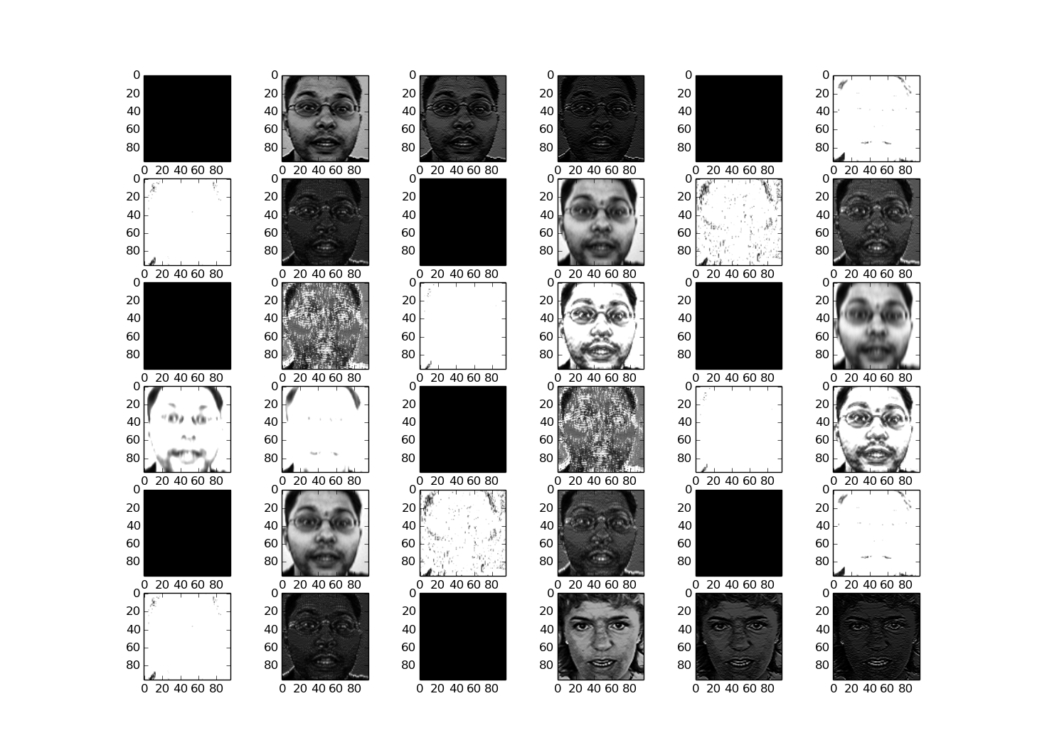
We see the input images

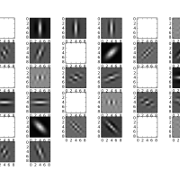
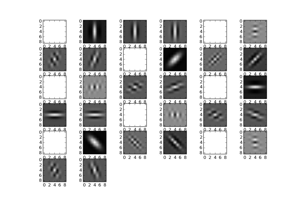
To visualize the 32 Gabor filters for the first input image, you see the filters
Look at the various outputs of the first image, when after convolving with 32 gabor filters (very interesting)
Here is the python code you are looking for. You will need the csv from kaggle facial keypoints competition.
import numpy as np
import pandas as pd
from numpy import genfromtxt
from numpy import ravel
import pylab as pl
from skimage import transform
import h5py
import cv2
from sklearn import cross_validation
import uuid
import random
from skimage import io, exposure, img_as_uint, img_as_float
from numpy import (array, dot, arccos)
from numpy.linalg import norm

df = pd.read_csv('test.csv',header=0)
df = df.dropna()

df['Image'] = df['Image'].apply(lambda im: np.fromstring(im, sep=' ') )
X = np.vstack (df['Image'].values)

X = X[:100].astype(np.uint8)
X = X.reshape(-1,96,96)


y = df.drop(['Image'], axis=1)
#y = y.interpolate()
y = y.values
y = y.astype(np.float32)
#y = y.reshape((-1,30))

print 'Input X,y:',X.shape, y.shape


def image_histogram_equalization(image, number_bins=256):
    # from http://www.janeriksolem.net/2009/06/histogram-equalization-with-python-and.html

    # get image histogram
    image_histogram, bins = np.histogram(image.flatten(), number_bins, normed=True)
    cdf = image_histogram.cumsum() # cumulative distribution function
    cdf = 255 * cdf / cdf[-1] # normalize

    # use linear interpolation of cdf to find new pixel values
    image_equalized = np.interp(image.flatten(), bins[:-1], cdf)

    return image_equalized.reshape(image.shape), cdf

def build_filters():
 filters = []
 ksize = 9
 for theta in np.arange(0, np.pi, np.pi / 8):
  for lamda in np.arange(0, np.pi, np.pi/4):
   kern = cv2.getGaborKernel((ksize, ksize), 1.0, theta, lamda, 0.5, 0, ktype=cv2.CV_32F)
   kern /= 1.5*kern.sum()
   filters.append(kern)
 return filters

def process(img, filters):
 accum = np.zeros_like(img)
 for kern in filters:
  fimg = cv2.filter2D(img, cv2.CV_8UC3, kern)
  np.maximum(accum, fimg, accum)
 return accum

filters = []
res = []
label = []

for k in xrange(len(X)):
 img = X[k]

 X[k, :, :] = image_histogram_equalization(X[k, :,:])[0]

 filters = build_filters()
 filters = np.asarray(filters)


 for i in xrange(len(filters)):
  res1 = process(img, filters[i])
  res.append(np.asarray(res1))


f = np.asarray(filters)
print 'Gabor Filters', f.shape
output = np.asarray(res)
label = np.asarray(label)
print 'Final output X,y', output.shape, label.shape


# Plot filters and convolved output

pl.figure()

# plot imagees
for k,im in enumerate(X[:36,:]):

 pl.subplot(6,6,k+1)
 pl.imshow(im.reshape(96,96), cmap='gray' )

pl.show()

# Convolved output
for k,im in enumerate(output[:36,:]):

 pl.subplot(6,6,k+1)
 pl.imshow(im.reshape(96,96), cmap='gray' )

pl.show()
# Show Filters

for k,im in enumerate(f[:32,:]):

 pl.subplot(6,6,k+1)
 pl.imshow(im.reshape(9,9), cmap='gray' )


pl.show()