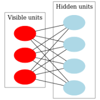
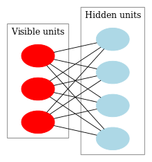
Restricted boltzmann machines commonly known as ‘RBM’s are excellent feature extractors, working just like autoencoders. They easily outperform PCA (principal component analysis) and LDA when it comes to dimensionality reduction techniques. The features extracted from images (eg MNIST) are fed to neural networks or machine learning algorithms such as SVM or Logistic regression classifiers. RBMs only work on inputs between 0 and 1 and even works very well on binary inputs. RBM are almost like NN except the rbm nodes are not connected to each other in the same layer.
I did various experiments using RBM and i was able to get 99% classification score on Olivetti faces and 98% on MNIST data. I converted the images to black and white (binary) images, fed these to RBM to do feature extraction to reduce the dimensionality and finally fed to the machine learning algorithm logistic regression. I never like machine learning algorithm running for days on large dataset, so by doing the dimensionality reduction and then feed these reduced data to classfier, gives the results within few minutes. For example, feeding the 28×28 pixel MNIST data has 784 dimensions and running SVM on 70,000 rows of data of 784 dimensions takes long hours to run, unless you have a supercomputer.
Let us give it a go on Olivetti faces and MNIST using RBM. Scikit provides a built in BernoulliRBM() built in function for python. You can rbm-notes of various observations showing some numbers for you to look at.
Olivetti faces
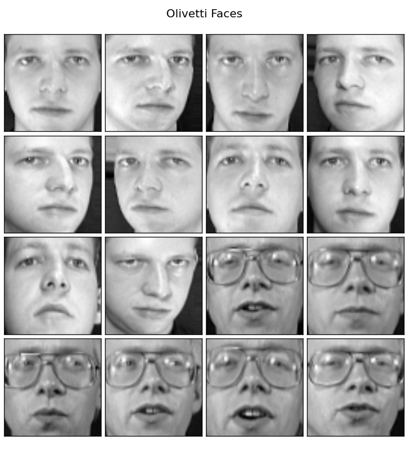
We will load the olivetti faces data in scikit. The data contains 64×64 pixel grayscale images of 400 rows. There are 40 classes and 10 faces of each person,
olivetti = datasets.fetch_olivetti_faces()
 X, Y = olivetti.data, olivetti.target
We will do some preprocessing, scaling between 0 and 1 of grayscale images
X = np.asarray( X, 'float32')
 X = (X - np.min(X, 0)) / (np.max(X, 0) + 0.0001)  # 0-1 scaling
We nudge the faces of 8×8 pixel patches and convolute. This produces 5 times the data. This means after this process our data size will be 400×5 = 2000 rows.
X, Y = nudge_dataset(X, Y)
[php]
def nudge_dataset(X, Y):
"""
This produces a dataset 5 times bigger than the original one,
by moving the 8×8 images in X around by 1px to left, right, down, up
"""
direction_vectors = [
[[0, 1, 0],
[0, 0, 0],
[0, 0, 0]],
[[0, 0, 0],
[1, 0, 0],
[0, 0, 0]],
[[0, 0, 0],
[0, 0, 1],
[0, 0, 0]],
[[0, 0, 0],
[0, 0, 0],
[0, 1, 0]]]
shift = lambda x, w: convolve(x.reshape((64, 64)), mode=’constant’,
weights=w).ravel()
X = np.concatenate([X] +
[np.apply_along_axis(shift, 1, X, vector)
for vector in direction_vectors])
Y = np.concatenate([Y for _ in range(5)], axis=0)
return X, Y
[/php]
then we convert the image array to binary (black and white). This is needed because RBM can extract features more efficiently on binary data, than on the grayscale data
# Convert image array to binary with threshold
X = X > 0.5
 Thats it, now our input data is ready, we setup bernoulli rbm and a logistic classifier using a pipeline. We extract top 180 components using the RBM and then we train it for 50 iterations.
logistic = linear_model.LogisticRegression(C=10)
rbm = BernoulliRBM(n_components=180, learning_rate=0.01, batch_size=10, n_iter=50, verbose=True, random_state=None)
clf = Pipeline(steps=[('rbm', rbm), ('clf', logistic)])
X_train, X_test, Y_train, Y_test = cross_validation.train_test_split( X, Y, test_size=0.2, random_state=0)
clf.fit(X_train,Y_train)
Y_pred = clf.predict(X_test)
print 'Score:  ',(metrics.classification_report(Y_test, Y_pred))
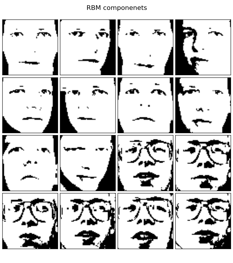
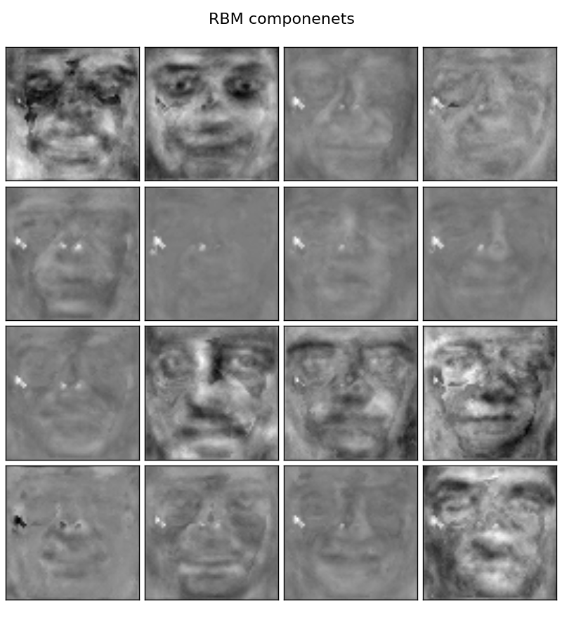
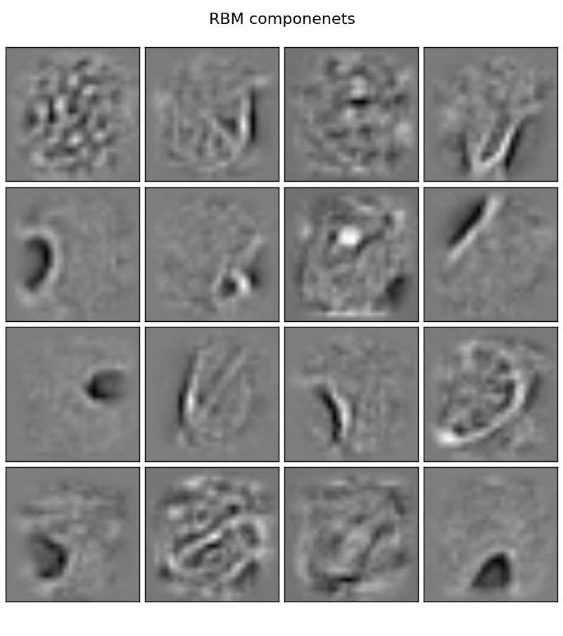
Now we plot the RBM components of first 16 faces
comp = rbm.components_
image_shape = (64, 64)
def plot_gallery(title, images, n_col, n_row):
    plt.figure(figsize=(2. * n_col, 2.26 * n_row))
    plt.suptitle(title, size=16)
    for i, comp in enumerate(images):
        plt.subplot(n_row, n_col, i + 1)
        vmax = max(comp.max(), -comp.min())
        plt.imshow(comp.reshape(image_shape), cmap=plt.cm.gray,
                   vmin=-vmax, vmax=vmax)
        plt.xticks(())
        plt.yticks(())
    plt.subplots_adjust(0.01, 0.05, 0.99, 0.93, 0.04, 0.)
    plt.show()
plot_gallery('RBM componenets', comp[:16], 4,4)
After running RBM, we see the extracted features on the first 16 faces. This looks similar like eigen face components..
As you can see from the graph, the optimal components with maximum variance is 140, yielding highest classification score of 98%.
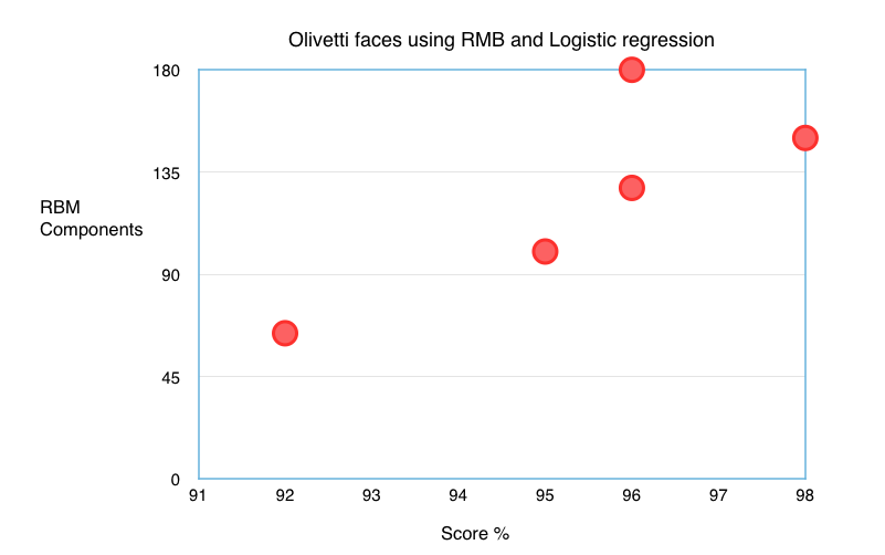
To push that score a bit, i did a Gridsearch to get the optimal parameters for logistic classifier of C=10 and the classification score jumped to 99%.
pipeline = Pipeline(steps=[('rbm', rbm), ('clf', logistic)])
parameters = {'clf__C': [0.001, 0.01, 0.1, 1, 10, 100, 1000] }
clf = grid_search.GridSearchCV (pipeline, parameters, n_jobs=-1, verbose=1)
print 'Grid search best:', clf.best_estimator_
Please note that this step will take a lot of time run.
99% score is not bad for the simple classifier just classifying black and white images. Great!
Let us move on to more complex handwriting recognition dataset MINST.
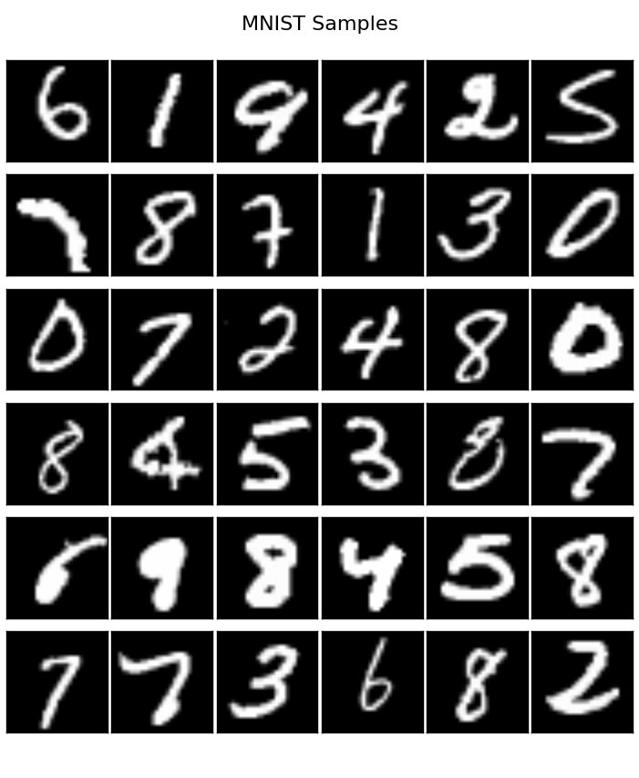
MINST data
MINST consist of 70,000 handwritten images each grayscale image is 28×28 which equals 784 dimensions. We do a dimensionality reduction with BernoulliRBM and then we will feed the features to a simple linear classifier, ie. logistic regression. This way it is fast.
mnist = datasets.fetch_mldata('MNIST original')
 X, Y = mnist.data, mnist.target
 X = np.asarray( X, 'float32')
 # Scaling between 0 and 1
 X = (X - np.min(X, 0)) / (np.max(X, 0) + 0.0001)  # 0-1 scaling
 # Convert to binary images
 X = X > 0.5
 print 'Input X shape', X.shape
Due to extensive computation required, we do not nudge and convolve, we just skip this step.
We setup a RBM with a simple classifier
rbm = BernoulliRBM(n_components=200, learning_rate=0.01, batch_size=10, n_iter=40, verbose=True, random_state=None)
logistic = linear_model.LogisticRegression(C=10)
clf = Pipeline(steps=[('rbm', rbm), ('clf', logistic)])
X_train, X_test, Y_train, Y_test = cross_validation.train_test_split( X, Y, test_size=0.2, random_state=0)
clf.fit(X_train, Y_train)
Y_pred = clf.predict(X_test)
print 'Score:  ',(metrics.classification_report(Y_test, Y_pred))
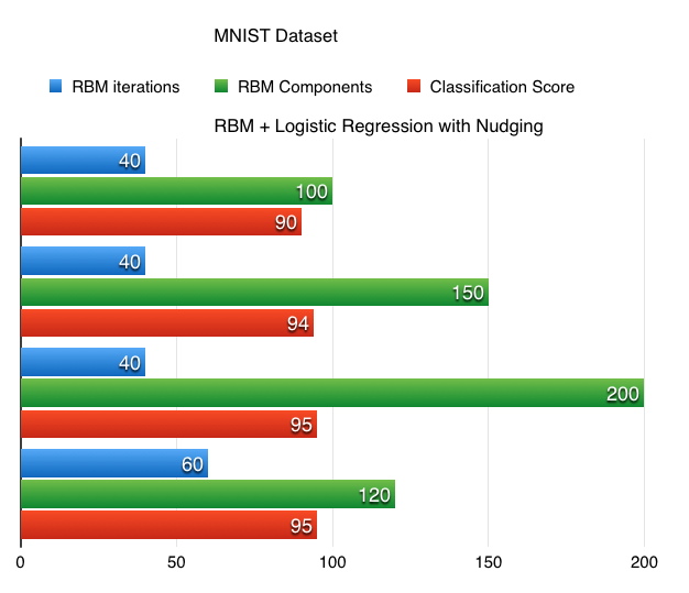
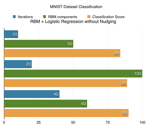
I was able to achieve 95% classification accuracy with MNIST using RBM+Logistic regression classifier and execution time is less than 5 minutes. On other note, i tried running SVM on rbm components on iMac, it took an awful long time so decided to settle with logistic regression.
The extracted RBM components of MNIST dataset look like this:
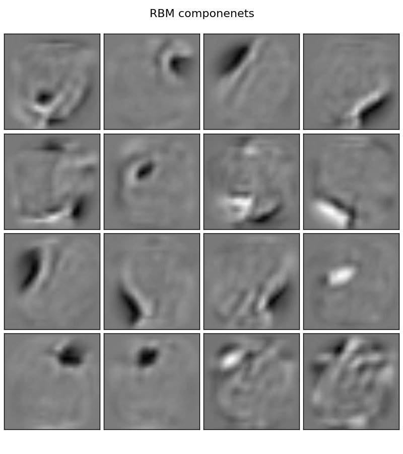
The learned RBM components (450) after 60 iterations look like this
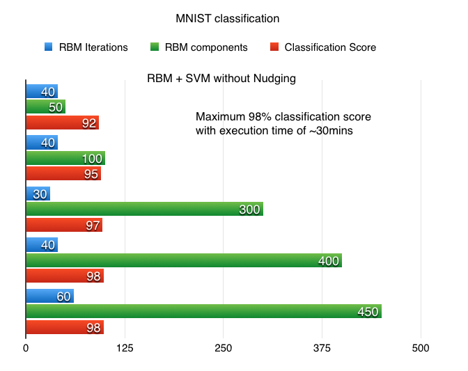
Support Vector Machines (SVM) work very well on large datasets. It only took a few minutes for the SVMs to bring the results on my imac. I was able to squeeze 98% classification score on MNIST after ~35 minutes of running time. It took 3 hours to run a GridSearch search to pull the optimal parameters.
sv = clf = svm.SVC(gamma=0.001, C=100.)
clf = Pipeline(steps=[('rbm', rbm), ('clf', sv)])
I trained both SVM and linear logistic regression classifiers and i noted down the observations. SVM clearly the winner with 98% classification score
Feed Forward Neural Network
Lets see how the neural network will perform on the MNIST dataset I trained a Pybrain feed forward neural network with backpropagation algorithm without using RBM. Here is what i did. I fed the original input to a neural network 784 inputs, 78 hidden and 10 outputs , it took a lot of time but i was only able to get test error of 11.1. This means on test data classification score by NN is 89.1, worse than SVM.
In the other experiment, i first trained a RBM and i assigned first RBM weights to the Input-Hidden weight connections. In my experiment it performed worse as i was able to get minimum error rate 19.1. One advantage is the NN is much faster on larget data set. From what i have learned, Deep Neural networks and Convolutional neural work excellent on images, whilst the error rate less than 1.0 on test data.
from pybrain.datasets            import ClassificationDataSet
from pybrain.utilities           import percentError
from pybrain.tools.shortcuts     import buildNetwork
from pybrain.supervised.trainers import BackpropTrainer
from pybrain.structure.modules   import SoftmaxLayer
from pybrain.tools.xml.networkwriter import NetworkWriter
from pybrain.tools.xml.networkreader import NetworkReader

from sklearn.neural_network import BernoulliRBM

import numpy as np
import pylab as pl
import pylab as plt

from sklearn import datasets
from sklearn import preprocessing
from numpy import ravel

from skimage import transform, filter

import os.path

# Plot faces
def plot_gallery(title, images, n_col, n_row):
    plt.figure(figsize=(2. * n_col, 2.26 * n_row))
    plt.suptitle(title, size=16)
    for i, comp in enumerate(images):
        plt.subplot(n_row, n_col, i + 1)
        vmax = max(comp.max(), -comp.min())
        plt.imshow(comp.reshape(image_shape), cmap=plt.cm.gray,
                   interpolation='nearest',
                   vmin=-vmax, vmax=vmax)
        plt.xticks(())
        plt.yticks(())
    plt.subplots_adjust(0.01, 0.05, 0.99, 0.93, 0.04, 0.)


# Load MNIST data

mnist = datasets.fetch_mldata('MNIST original')
x, y = mnist.data, mnist.target

X = []
for i in xrange(len(x)):
 X.append ( ravel(transform.resize (x[i].reshape(28,28) , (16,16))) )

X = np.asarray(X, 'float32')

X = (X - np.min(X, 0)) / (np.max(X, 0) + 0.0001)


#X = X > 0.52
# Shrink the size of images to smaller ones

print 'MNIST data:', X.shape

rbm = BernoulliRBM(n_components=30, learning_rate=0.01, batch_size=10, n_iter=50, verbose=True, random_state=None)
rbm.fit(X)

rbmweights = rbm.components_[0]

print 'RBM weights shape', rbmweights.shape
# Training data

trds = ClassificationDataSet(256 , 1 , nb_classes=10)

for k in xrange(0,65000):
  trds.addSample(X[k],y[k])

# Test data set

tsds = ClassificationDataSet(256 , 1 , nb_classes=10)

for k in xrange(65000,70000):
 tsds.addSample(X[k],y[k])

tsds._convertToOneOfMany( )
trds._convertToOneOfMany( )

fnn = buildNetwork(trds.indim, 32 , trds.outdim, outclass=SoftmaxLayer)

trainer = BackpropTrainer(fnn, dataset=trds, momentum=0.9 , learningrate=0.25, verbose=True, weightdecay=0.01)

print 'NN Params length', len(fnn.params)

hid2out = np.full( len(fnn.params) - len(rbmweights),1)
#hid2out = np.random.uniform( -1,1,len(fnn.params) - len(rbmweights))
nn_weights = np.concatenate((rbmweights,hid2out),axis=0)

print 'New Params weights:', len(nn_weights)

fnn._setParameters(nn_weights)

trainer.trainEpochs(20)

print 'Train Error: ' , percentError( trainer.testOnClassData (
            )
           , trds['class'] )

print 'Test Error: ' , percentError( trainer.testOnClassData (
           dataset=tsds )
           , tsds['class'] )


#NetworkWriter.writeToFile(fnn, 'mnist.xml')