Facial keypoints extraction is a challenging problem and deep learning is a hot topic and much explored area. Caffe is a popular deep learning library implementing deep learning on large datasets. Caffe is much much faster and convolutional neural networks seems to perform much better with images and can run in GPU and CPU. Running in Nvidia GPU with CUDA support is almost 20X faster than CPU. MNIST dataset classification has achieved more than 99% accuracy using convolutions in images.
The facial keypoints problem is a classic multi label regression problem. The input is (96,96) pixel grayscale images and we have to determine 30 outputs. Kaggle has a interesting facial keypoints competition: https://www.kaggle.com/c/facial-keypoints-detection
Before we move on to using caffe, lets try a simple linear regression model, to see if we can crack this problem with lowest MSE (mean square error). We will use FANN neural network library written in C as native C code is so much faster is todays CPUs than python.
What do you need
Before we proceed further, you must be familiar with
Python
Pandas
C/C++
Scikit-learn, Scikit-Image
Numpy/Scipy
CUDA from Nvidia
Linux (ubuntu)
Compiling various tools and libraries in Linux/Mac
Basic knowledge of Caffe and Deep Learning
FANN Neural Network Library
Implementing a neural network using FANN is the easiest i have seen. You can find the documentation here: http://leenissen.dk/fann/html/files/fann_train-h.html
All you have to do is dump the image data, into the format FANN is able to read and the netowrk model will be able to learn in this format. We reduce and shrink the images to 28×28 pixels and dump the data for our network to read. We use 100% of the training data without dropping the NaNs and we populate it with mean values.
A simple linear regression using FANN neural network perceptron model. after about 100 iterations produces only MSE of 0.000146. All i did was to connect inputs 24*24 size images (shrinked by 4X) to 30 outputs.
 Epochs          980. Current error: 0.0001471710. Bit fail 0.
 Epochs          990. Current error: 0.0001470396. Bit fail 0.
 Epochs         1000. Current error: 0.0001469008. Bit fail 0.
As you can see, the real training error is 0.000146 * 96 * 4 = 0.056
You can find all the files in github project https://github.com/olddocks/facialkeypoints. You have to download the kaggle csv files as well.
prepare_test.py  -> Dumps the images as training data for FANN to read
 prepare_train.py -> Prepares and dumps the test data to FANN format
 facial.c -> Neural network trainer
 ftest.c -> Testing and predictions (produces results.txt)
 kaggle.py -> Produces kaggle.csv (results to upload to kaggle)
To start the trainer, first you have to first compile the C code.
gcc facial.c -o facial -lfann2 -lm -I /usr/local/include/fann
gcc ftest.c -o ftest -lfann2 -lm -I /usr/local/include/fann
After you run
python prepare_data.py
python prepare_test.py
./facial
./ftest
python kaggle.py
Lets analyze the results are like this first test images 1,2. The first shows 30 predicted against the original values. The one in brackets are difference between predicted and original, just for the understanding on how far the difference is..
Testing network..
0  69.45/71.08(1.63)  38.68/39.58(0.91)  28.68/26.33(-2.35)  37.64/38.05(0.42)  59.64/59.26(-0.39)  36.75/36.07(-0.68)  74.55/73.94(-0.61)  35.51/34.62(-0.89)  36.81/37.48(0.67)  39.01/39.40(0.39)  21.39/22.06(0.67)  39.60/40.33(0.73)  54.88/53.30(-1.58)  29.95/29.99(0.04)  81.32/80.95(-0.37)  28.47/27.98(-0.49)  38.53/38.78(0.25)  32.26/33.30(1.04)  14.30/14.80(0.50)  33.95/35.98(2.04)  49.06/47.37(-1.69)  65.84/69.80(3.96)  70.50/72.60(2.10)  73.40/71.86(-1.54)  32.93/34.23(1.30)  77.32/77.34(0.02)  50.59/51.60(1.01)  75.66/75.96(0.31)  48.09/46.98(-1.11)  82.92/81.27(-1.64)
1 64.18/64.40(0.22) 36.78/38.50(1.73) 30.59/29.44(-1.15) 39.62/39.95(0.33) 59.07/59.26(0.19) 37.45/36.07(-1.38) 72.72/73.94(1.23) 36.10/34.62(-1.47) 37.28/37.48(0.20) 39.42/39.40(-0.02) 23.08/22.06(-1.02) 39.85/40.33(0.48) 54.15/53.30(-0.85) 31.38/29.99(-1.39) 78.95/80.95(1.99) 29.59/27.98(-1.61) 38.57/38.78(0.21) 33.13/33.30(0.17) 16.28/14.80(-1.49) 34.13/35.98(1.85) 46.06/46.74(0.68) 61.04/63.73(2.69) 68.53/72.60(4.07) 74.52/71.86(-2.65) 34.41/34.23(-0.18) 77.68/77.34(-0.34) 50.34/51.60(1.25) 75.32/75.96(0.64) 47.66/48.18(0.52) 76.92/75.27(-1.65)
2  68.75/69.26(0.51)  38.35/40.36(2.01)  29.91/28.49(-1.42)  35.56/36.19(0.63)  59.29/59.26(-0.03) 36.69/36.07(-0.63)  74.89/73.94(-0.95)  35.78/34.62(-1.16)  36.97/37.48(0.51)  38.88/39.40(0.52)  21.42/22.06(0.64)  39.23/40.33(1.10)  54.13/53.30(-0.83)  30.54/29.99(-0.55)  81.75/80.95(-0.80)  28.97/27.98(-0.99)  38.69/38.78(0.09)  32.46/33.30(0.85)  14.35/14.80(0.45)  34.06/35.98(1.92)  46.11/45.83(-0.29)  65.68/75.67(9.99)  69.40/72.60(3.20)  74.28/71.86(-2.41)  33.11/34.23(1.13)  77.40/77.34(-0.06)  49.99/51.60(1.61)  76.66/75.96(-0.70)  46.23/45.18(-1.04)  80.29/84.98(4.69)
Mean Test Square Error: 0.000166
I uploaded these results to kaggle and it give mean top 16 position with 3.3 error. Wow! Not bad 🙂
P.S: I have played with this dataset using multiple neuron layers to get maximum accuracy by implementing multiple hidden layers. It seems perceptron model performed the best as far as the problem goes.
Deep Learning
Deep learning is made up multiple layers convolution and pooling layers (which are like feature extractors), finally followed by fully connected layers (IP) which in turn connects to output. The multiple pooling and convolution layers also a technique to reduce the dimensionality of images. A good tutorial is found here: http://ufldl.stanford.edu/tutorial/supervised/ConvolutionalNeuralNetwork/
We will see how caffe performs and extract the facial keypoints by running a DNN in a GPU. I have used nvidia 750ti GPU with CUDA installed in a ubuntu system.
Lets say if the image dimensions are (M,N), each convolution layer with kernel size (x,y) produces (M-x+1, N-y+1) with number of outputs. Pooling greatly bifurcates the pixel size. After each pooling with kernel size K x K, the resulting size becomes (M/k, N/k) with number of outputs
This is what we do..
1. Import the images from kaggle CSV, we drop NaNs and do preprocessing between 0 and 1 (divide by 255) for input and output labels (divide by 96), then equalize the histogram and finally dump the numpy array of the input and output labels to HDF5 files.
X is input and y is output label shape
Input Train, Test shapes (X,y): (1600, 1, 96, 96) (1600, 30) (540, 1, 96, 96) (540, 30)
2. We write a layer file with convolution and pooling layers and also a solver file with EUCLIDEAN_LOSS with 30 outputs for caffe.
3. Train the caffe and and finally predict the outputs by loading chunks of data (64 batches) into MEMORY_LAYER. This way the model can run into a small PCs with atleast 2GB of memory size.
4. To make the model more accurate, we also give the model more 15 extra features like computing euclidean distances from nose to eyes, two eye centers etc.
5. We specify RELU (to allow values > 0, plus faster converging) , Dropout layer to prevent overfitting.
6. We can calculate distances in facial points and give them as feature vector to the learning model. We will save it for later, but lets see how our small model works..
See the my git project: https://github.com/olddocks/caffe-facialkp
This is how you run the project.
python fkp.py
 ./facialkp
 python output.py
The following is a brief description of the files in the project and how to use them
fkp.py -> to write and prepare all data to hd5
./facialkp -> Run the caffe model
output.py -> Predict and plot graphs in simple 64 batches. it writes into csv
solver.prototxt – > Edit this for maximum iterations, gamma, learning rate etc.
facialkp.prototxt -> Layer file for training
facialkp_predict -> Layer file for predictions
kaggle.py -> writes kaggle output to upload (you have manually edit csv files to add header labels, if not it will not work. Sorry i am a lazy coder :()
Our 4D data dimensions
Input data (1600,1,96,96) -> Channel 1 for grayscale images
Output labels (1600,30)
Our solver.prototxt, we specify GPU/CPU
net: "/home/pbu/Desktop/facialkp.prototxt"
test_iter: 6
test_interval: 100
base_lr: 0.01
lr_policy: "fixed"
weight_decay: 0.01
stepsize: 300
gamma: 0.1
display: 100
max_iter: 2000
momentum: 0.9
snapshot: 1000
snapshot_prefix: "/home/pbu/Desktop/tmp"
solver_mode: GPU
Update: Please note i have discovered that IP layer and convolutional layers produce unexpected strange results because of the bias and weights are not initialized properly. You will need to include this code in your layer file
weight_filler {
      type: "xavier"
    }
    bias_filler {
      type: "constant"
    }
Our training layer file
name: "FKPReg"
layers {
  name: "fkp"
  top: "data"
  top: "label"
  type: HDF5_DATA
  hdf5_data_param {
   source: "train.txt"
   batch_size: 64
  }
    include: { phase: TRAIN }
}
layers {
  name: "data"
  type: HDF5_DATA
  top: "data"
  top: "label"
  hdf5_data_param {
    source: "test.txt"
    batch_size: 100
  }
  include: { phase: TEST }
}
layers {
  name: "conv1"
  type: CONVOLUTION
  bottom: "data"
  top: "conv1"
  convolution_param {
    num_output: 32
    kernel_size: 11
    stride: 2
    bias_filler {
      type: "constant"
      value: 0.1
    }
  }
}
layers {
  name: "relu2"
  type: RELU
  bottom: "conv1"
  top: "conv1"
}
layers {
  name: "pool1"
  type: POOLING
  bottom: "conv1"
  top: "pool1"
  pooling_param {
    pool: MAX
    kernel_size: 2
    stride: 2
  }
}
layers {
  name: "conv2"
  type: CONVOLUTION
  bottom: "pool1"
  top: "conv2"
  convolution_param {
    num_output: 64
    pad: 2
    kernel_size: 7
    group: 2
       bias_filler {
      type: "constant"
      value: 0.1
    }
  }
}
layers {
  name: "relu2"
  type: RELU
  bottom: "conv2"
  top: "conv2"
}
layers {
  name: "pool2"
  type: POOLING
  bottom: "conv2"
  top: "pool2"
  pooling_param {
    pool: MAX
    kernel_size: 2
    stride: 2
  }
}
layers {
  name: "norm2"
  type: LRN
  bottom: "pool2"
  top: "norm2"
  lrn_param {
    norm_region: WITHIN_CHANNEL
    local_size: 3
    alpha: 5e-05
    beta: 0.75
  }
}
layers {
  name: "conv3"
  type: CONVOLUTION
  bottom: "norm2"
  top: "conv3"
  convolution_param {
    num_output: 32
    pad: 1
    kernel_size: 5

    bias_filler {
      type: "constant"
      value: 0.1
    }
  }
}
layers {
  name: "relu3"
  type: RELU
  bottom: "conv3"
  top: "conv3"
}

layers {
  name: "conv4"
  type: CONVOLUTION
  bottom: "conv3"
  top: "conv4"
  convolution_param {
    num_output: 64
    pad: 1
    kernel_size: 5
    bias_filler {
      type: "constant"
      value: 0.1
    }
  }
}
layers {
  name: "relu4"
  type: RELU
  bottom: "conv4"
  top: "conv4"
}
layers {
  name: "conv5"
  type: CONVOLUTION
  bottom: "conv4"
  top: "conv5"
  convolution_param {
    num_output: 32
    pad: 1
    kernel_size: 5
        bias_filler {
      type: "constant"
      value: 0.1
    }
  }
}
layers {
  name: "relu5"
  type: RELU
  bottom: "conv5"
  top: "conv5"
}
layers {
  name: "pool5"
  type: POOLING
  bottom: "conv5"
  top: "pool5"
  pooling_param {
    pool: MAX
    kernel_size: 4
    stride: 2
  }
}
layers {
  name: "drop0"
  type: DROPOUT
  bottom: "pool5"
  top: "pool5"
  dropout_param {
    dropout_ratio: 0.5
  }
}
layers {
  name: "ip1"
  type: INNER_PRODUCT
  bottom: "pool5"
  top: "ip1"
  inner_product_param {
    num_output: 100
        bias_filler {
      type: "constant"
      value: 0.1
    }
  }
}
layers {
  name: "relu4"
  type: RELU
  bottom: "ip1"
  top: "ip1"
}
layers {
  name: "drop1"
  type: DROPOUT
  bottom: "ip1"
  top: "ip1"
  dropout_param {
    dropout_ratio: 0.5
  }
}
layers {
  name: "ip2"
  type: INNER_PRODUCT
  bottom: "ip1"
  top: "ip2"
  inner_product_param {
    num_output: 30
    weight_filler {
    type="xavier"
    }
    bias_filler {
      type: "constant"
      value: 0.1
    }
  }
}
layers {
  name: "relu22"
  type: RELU
  bottom: "ip2"
  top: "ip2"
}
layers {
  name: "loss"
  type: EUCLIDEAN_LOSS
  bottom: "ip2"
  bottom: "label"
  top: "loss"
}
We run caffe and we see output like this. We can clearly see how convolution and pool layers shape the data.
I0223 18:26:03.296244  3233 net.cpp:67] Creating Layer data
 I0223 18:26:03.296267  3233 net.cpp:356] data -> data
 I0223 18:26:03.296294  3233 net.cpp:356] data -> label
 I0223 18:26:03.296316  3233 net.cpp:96] Setting up data
 I0223 18:26:03.296334  3233 hdf5_data_layer.cpp:57] Loading filename from test.txt
 I0223 18:26:03.296385  3233 hdf5_data_layer.cpp:69] Number of files: 1
 I0223 18:26:03.296402  3233 hdf5_data_layer.cpp:29] Loading HDF5 filefacialkp-test.hd5
 I0223 18:26:03.498864  3233 hdf5_data_layer.cpp:49] Successully loaded 540 rows
 I0223 18:26:03.498987  3233 hdf5_data_layer.cpp:81] output data size: 100,1,96,96
 I0223 18:26:03.499011  3233 net.cpp:103] Top shape: 100 1 96 96 (921600)
 I0223 18:26:03.499032  3233 net.cpp:103] Top shape: 100 45 1 1 (4500)
 I0223 18:26:03.499068  3233 net.cpp:67] Creating Layer conv1
 I0223 18:26:03.499091  3233 net.cpp:394] conv1 <- data
 I0223 18:26:03.499119  3233 net.cpp:356] conv1 -> conv1
 I0223 18:26:03.499153  3233 net.cpp:96] Setting up conv1
 I0223 18:26:03.499348  3233 net.cpp:103] Top shape: 100 64 44 44 (12390400)
 I0223 18:26:03.499392  3233 net.cpp:67] Creating Layer relu1
 I0223 18:26:03.499411  3233 net.cpp:394] relu1 <- conv1
 I0223 18:26:03.499433  3233 net.cpp:345] relu1 -> conv1 (in-place)
 I0223 18:26:03.499455  3233 net.cpp:96] Setting up relu1
 I0223 18:26:03.499476  3233 net.cpp:103] Top shape: 100 64 44 44 (12390400)
 I0223 18:26:03.499498  3233 net.cpp:67] Creating Layer pool1
 I0223 18:26:03.499516  3233 net.cpp:394] pool1 <- conv1
 I0223 18:26:03.499536  3233 net.cpp:356] pool1 -> pool1
 I0223 18:26:03.499557  3233 net.cpp:96] Setting up pool1
 I0223 18:26:03.499583  3233 net.cpp:103] Top shape: 100 64 22 22 (3097600)
 I0223 18:26:03.499615  3233 net.cpp:67] Creating Layer conv2
 I0223 18:26:03.499632  3233 net.cpp:394] conv2 <- pool1
 I0223 18:26:03.499654  3233 net.cpp:356] conv2 -> conv2
 I0223 18:26:03.499677  3233 net.cpp:96] Setting up conv2
 I0223 18:26:03.500277  3233 net.cpp:103] Top shape: 100 64 22 22 (3097600)
 I0223 18:26:03.500363  3233 net.cpp:67] Creating Layer relu2
 I0223 18:26:03.500388  3233 net.cpp:394] relu2 <- conv2
 I0223 18:26:03.500412  3233 net.cpp:345] relu2 -> conv2 (in-place)
 I0223 18:26:03.500438  3233 net.cpp:96] Setting up relu2
 I0223 18:26:03.500460  3233 net.cpp:103] Top shape: 100 64 22 22 (3097600)
 I0223 18:26:03.500483  3233 net.cpp:67] Creating Layer pool2
 I0223 18:26:03.500500  3233 net.cpp:394] pool2 <- conv2
 I0223 18:26:03.500521  3233 net.cpp:356] pool2 -> pool2
 I0223 18:26:03.500545  3233 net.cpp:96] Setting up pool2
 I0223 18:26:03.500569  3233 net.cpp:103] Top shape: 100 64 11 11 (774400)
 I0223 18:26:03.500591  3233 net.cpp:67] Creating Layer relu3
 I0223 18:26:03.500607  3233 net.cpp:394] relu3 <- pool2
 I0223 18:26:03.500627  3233 net.cpp:345] relu3 -> pool2 (in-place)
 I0223 18:26:03.500648  3233 net.cpp:96] Setting up relu3
 I0223 18:26:03.500669  3233 net.cpp:103] Top shape: 100 64 11 11 (774400)
 I0223 18:26:03.500694  3233 net.cpp:67] Creating Layer conv3
 I0223 18:26:03.500711  3233 net.cpp:394] conv3 <- pool2
 I0223 18:26:03.500732  3233 net.cpp:356] conv3 -> conv3
 I0223 18:26:03.500756  3233 net.cpp:96] Setting up conv3
 I0223 18:26:03.501147  3233 net.cpp:103] Top shape: 100 128 11 11 (1548800)
 I0223 18:26:03.501216  3233 net.cpp:67] Creating Layer pool3
 I0223 18:26:03.501240  3233 net.cpp:394] pool3 <- conv3
 I0223 18:26:03.501266  3233 net.cpp:356] pool3 -> pool3
 I0223 18:26:03.501291  3233 net.cpp:96] Setting up pool3
 I0223 18:26:03.501317  3233 net.cpp:103] Top shape: 100 128 6 6 (460800)
 I0223 18:26:03.501343  3233 net.cpp:67] Creating Layer relu4
 I0223 18:26:03.501359  3233 net.cpp:394] relu4 <- pool3
 I0223 18:26:03.501379  3233 net.cpp:345] relu4 -> pool3 (in-place)
 I0223 18:26:03.501399  3233 net.cpp:96] Setting up relu4
 I0223 18:26:03.501421  3233 net.cpp:103] Top shape: 100 128 6 6 (460800)
 I0223 18:26:03.501446  3233 net.cpp:67] Creating Layer conv4
 I0223 18:26:03.501463  3233 net.cpp:394] conv4 <- pool3
 I0223 18:26:03.501485  3233 net.cpp:356] conv4 -> conv4
 I0223 18:26:03.501515  3233 net.cpp:96] Setting up conv4
 I0223 18:26:03.501665  3233 net.cpp:103] Top shape: 100 100 8 8 (640000)
 I0223 18:26:03.501701  3233 net.cpp:67] Creating Layer drop0
 I0223 18:26:03.501719  3233 net.cpp:394] drop0 <- conv4
 I0223 18:26:03.501739  3233 net.cpp:345] drop0 -> conv4 (in-place)
 I0223 18:26:03.501761  3233 net.cpp:96] Setting up drop0
 I0223 18:26:03.501780  3233 net.cpp:103] Top shape: 100 100 8 8 (640000)
 I0223 18:26:03.501801  3233 net.cpp:67] Creating Layer ip1
 I0223 18:26:03.501818  3233 net.cpp:394] ip1 <- conv4
 I0223 18:26:03.501839  3233 net.cpp:356] ip1 -> ip1
 I0223 18:26:03.501924  3233 net.cpp:96] Setting up ip1
 I0223 18:26:03.505934  3233 net.cpp:103] Top shape: 100 100 1 1 (10000)
 I0223 18:26:03.506044  3233 net.cpp:67] Creating Layer relu5
 I0223 18:26:03.506064  3233 net.cpp:394] relu5 <- ip1
 I0223 18:26:03.506088  3233 net.cpp:345] relu5 -> ip1 (in-place)
 I0223 18:26:03.506110  3233 net.cpp:96] Setting up relu5
 I0223 18:26:03.506141  3233 net.cpp:103] Top shape: 100 100 1 1 (10000)
 I0223 18:26:03.506165  3233 net.cpp:67] Creating Layer drop1
 I0223 18:26:03.506181  3233 net.cpp:394] drop1 <- ip1
 I0223 18:26:03.506199  3233 net.cpp:345] drop1 -> ip1 (in-place)
 I0223 18:26:03.506218  3233 net.cpp:96] Setting up drop1
 I0223 18:26:03.506237  3233 net.cpp:103] Top shape: 100 100 1 1 (10000)
 I0223 18:26:03.506265  3233 net.cpp:67] Creating Layer ip2
 I0223 18:26:03.506281  3233 net.cpp:394] ip2 <- ip1
 I0223 18:26:03.506302  3233 net.cpp:356] ip2 -> ip2
 I0223 18:26:03.506325  3233 net.cpp:96] Setting up ip2
 I0223 18:26:03.506366  3233 net.cpp:103] Top shape: 100 60 1 1 (6000)
 I0223 18:26:03.506391  3233 net.cpp:67] Creating Layer relu6
 I0223 18:26:03.506407  3233 net.cpp:394] relu6 <- ip2
 I0223 18:26:03.506425  3233 net.cpp:345] relu6 -> ip2 (in-place)
 I0223 18:26:03.506445  3233 net.cpp:96] Setting up relu6
 I0223 18:26:03.506464  3233 net.cpp:103] Top shape: 100 60 1 1 (6000)
 I0223 18:26:03.506484  3233 net.cpp:67] Creating Layer drop3
 I0223 18:26:03.506500  3233 net.cpp:394] drop3 <- ip2
 I0223 18:26:03.506520  3233 net.cpp:345] drop3 -> ip2 (in-place)
 I0223 18:26:03.506538  3233 net.cpp:96] Setting up drop3
 I0223 18:26:03.506554  3233 net.cpp:103] Top shape: 100 60 1 1 (6000)
 I0223 18:26:03.506575  3233 net.cpp:67] Creating Layer ip3
 I0223 18:26:03.506592  3233 net.cpp:394] ip3 <- ip2
 I0223 18:26:03.506611  3233 net.cpp:345] ip3 -> ip2 (in-place)
 I0223 18:26:03.506631  3233 net.cpp:96] Setting up ip3
 I0223 18:26:03.506662  3233 net.cpp:103] Top shape: 100 45 1 1 (4500)
 I0223 18:26:03.506687  3233 net.cpp:67] Creating Layer loss
 I0223 18:26:03.506703  3233 net.cpp:394] loss <- ip2
 I0223 18:26:03.506721  3233 net.cpp:394] loss <- label
 I0223 18:26:03.506742  3233 net.cpp:356] loss -> loss
 I0223 18:26:03.506762  3233 net.cpp:96] Setting up loss
 I0223 18:26:03.506783  3233 net.cpp:103] Top shape: 1 1 1 1 (1)
 I0223 18:26:03.506799  3233 net.cpp:109]     with loss weight 1
Finally, train and test error which is 0.029*96 = 2.7, which is too high and the network is not converging and seems to learn only a bit.
I0223 19:10:08.230324  3702 solver.cpp:342] Snapshotting solver state to /home/pbu/Desktop/tmp_iter_1000.solverstate
 I0223 19:10:08.234257  3702 solver.cpp:264] Iteration 1000, Testing net (#0)
 I0223 19:10:08.384732  3702 solver.cpp:315] Test net output #0: loss = 0.0294809 (* 1 = 0.0294809 loss)
It shows that we get test error 0.029. We multiply by 96 (because we normalized it) and the result is 2.7 error, Wow, much better than the simple fann model. But wait? is it overfitting, you will know when you validate the answers with kaggle.
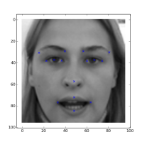
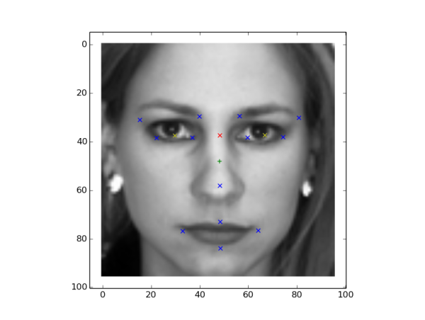
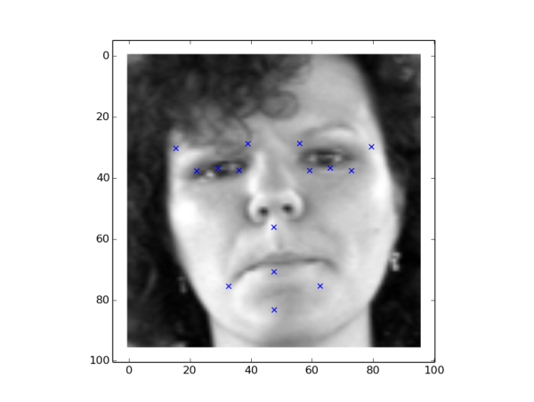
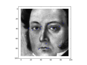
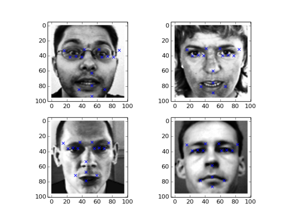
Lets take a look at the couple of predicted outputs from kaggle test set 0-64
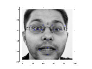
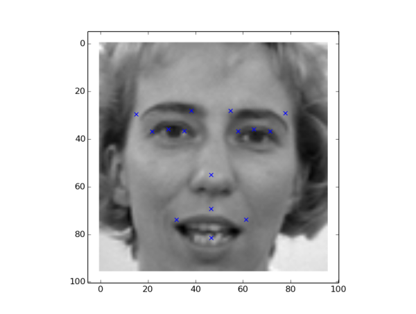
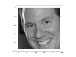
Lets take a look at Set 100-164 (bit of orientation and tilt)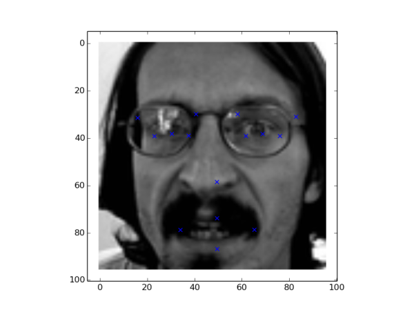
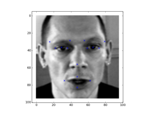
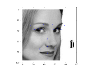
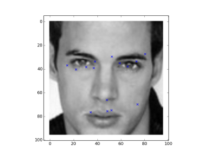
Lets take a look at the test set 200-264 (it gets more complex) and more errors in predictions.
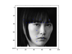
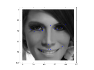
Now more complicated images in set 400-644, flipped right and left and our model is not doing good with respect to orientation and angles of faces.
I uploaded the results to Kaggle and i got final prediction error loss of 4.6. Looks like our simple FANN model with 3.3 blows away the Deep learning with test error 2.7?
Why do you think our caffe model performing poorly? One of the reasons is because we dropped 70% of the training data because of the NaNs. We must use the data by filling up the mean and may be the error loss will improve.
So far we used the dataset dropping all NaNs. Lets see we use 100% of the dataset and see if there is any improvement in the model. We interpolate the mean values of the missing values and train the model. You can make changes in fkp.py
Train (X,y): (6000, 1, 96, 96) (6000, 30)
Test (X,y) : (1049, 1, 96, 96) (1049, 30)
After 1000 iterations, with learning rate of 0.01
I0224 19:10:10.937978 3639 solver.cpp:246] Iteration 1000, loss = 0.0102475
I0224 19:10:10.938068 3639 solver.cpp:264] Iteration 1000, Testing net (#0)
I0224 19:10:11.084893 3639 solver.cpp:315] Test net output #0: loss = 0.00789451 (* 1 = 0.00789451 loss)
After 1000 iterations, the test error is 0.00789 multiplied by 96 = 0.75, looks very minimum error compared to 2.7 (with small dataset). Lets not get fooled by the model. Let plot the x,y predictions and see if it is accurate
Looking the plots, the model predictions are far worse than the previous ones, despite a low test error.
From my observations the most accurate model was dataset created by dropping NaNs, with 500 iterations of learning rate of 0.01 (see below). Too fast learning makes the model to converge to mean which means the model is memorizing the mean. I could only squeeze to get kaggle result of 4.4 of the caffe model.
All the code files can be accessed at
Facial keypoints Fann library: https://github.com/olddocks/facialkeypoints
Deep learning in Caffe: https://github.com/olddocks/caffe-facialkp
A much better approach to facial points extraction model documented by Daniel Nouri and has high accuracy http://danielnouri.org/notes/2014/12/17/using-convolutional-neural-nets-to-detect-facial-keypoints-tutorial/
Caffe has a google public group for discussions. You can ask questions there as caffe lacks full documentation on regression and other topics: https://groups.google.com/forum/#!forum/caffe-users

